6 Code
We aim to determine the optimal policy using bandit algorithms. We will focus on Nvidia and AT&T assets, seeking to maximize rewards while minimizing risk. Our simulation will span 100 days, with an initial capital of $100,000. We will compare the portfolio’s performance against a no-risk benchmark simulation.
import numpy as np
import matplotlib.pyplot as plt
from scipy.stats import lognorm
# Function to sample from a log-normal distribution for the returns
def sample_dynamic_return(mu, sigma):
"""Sample a value from a log-normal distribution with changing parameters."""
return np.random.lognormal(mean=mu, sigma=sigma)
# Cost function calculation: Expected return + Risk (variance + covariance)
def cost_function(risky_proportions, r, sigma, covariance_matrix):
"""
Calculate the cost for portfolio optimization, considering only risky assets.
Args:
risky_proportions (ndarray): Proportions of the risky assets at step i-1.
r (ndarray): Returns at step i.
covariance_matrix (ndarray): Covariance matrix of asset returns.
Returns:
float: The total cost.
"""
# No-risk asset proportion is the remainder of 1 - sum(risky_proportions)
no_risk_proportion = 1 - np.sum(risky_proportions)
# Portfolio weights (risky assets only for the decision-making)
weights = np.concatenate([risky_proportions, [no_risk_proportion]])
# First term: Expected return (weighted sum of returns)
expected_return = np.dot(weights, r)
# Second term: Portfolio risk (variance + covariance) using the risky assets only
portfolio_risk = 0.5 * np.dot(risky_proportions,sigma- np.dot(covariance_matrix, risky_proportions))
# Total cost
return expected_return + portfolio_risk
# Bandit algorithm with dynamic portfolio optimization (using cost function)
def bandit_algorithm_with_dynamic_returns(stock_params, no_risk_return, initial_money, num_steps, epsilon, covariance_matrix, verbose=True):
"""
Bandit algorithm for dynamic portfolio allocation considering a cost function.
Args:
stock_params (list of tuples): Each tuple contains (mu, sigma) for a stock's log-normal distribution.
no_risk_return (float): Fixed return of the no-risk asset.
initial_money (float): Initial amount of money to allocate.
num_steps (int): Number of steps in the simulation.
epsilon (float): Exploration probability.
covariance_matrix (ndarray): Covariance matrix for the assets.
verbose (bool): Whether to log actions and rewards at each step.
Returns:
portfolio_value (list): Portfolio value over time.
total_rewards (list): Total rewards (portfolio return) over time.
allocations (list): Allocations of money at each step.
Q (ndarray): Final estimated values for each asset.
"""
num_risky_assets = len(stock_params) # Number of risky assets
num_assets = num_risky_assets + 1 # Including the no-risk asset
Q = np.zeros(num_assets) # Estimated rewards for each arm
N = np.zeros(num_assets) # Number of times each arm is selected
portfolio_value = [initial_money] # Store portfolio value over time
total_rewards = [0] # Store total rewards over time (portfolio return)
allocations = [] # Store allocations at each step
for step in range(num_steps):
# Epsilon-greedy action selection
if np.random.random() < epsilon:
proportions = np.random.dirichlet(np.ones(num_assets), size=1).flatten() # Explore
else:
proportions = np.zeros(num_assets)
best_action = np.argmax(Q)
proportions[best_action] = 1 # Exploit, allocate everything to the best action
# Ensure risky proportions sum to 1
proportions = proportions / proportions.sum()
risky_proportions = [proportions[0],proportions[1]]
# Sample new returns for each asset (risky assets and no-risk asset)
rewards = np.zeros(num_assets)
for i in range(num_risky_assets):
mu, sigma = stock_params[i]
rewards[i] = sample_dynamic_return(mu, sigma)-1 # Risky assets: sample dynamic returns
s = [float(stock_params[0][1])**2,float(stock_params[1][1])**2]
print(step, rewards, '\n')
# The no-risk asset has a fixed return
rewards[-1] = no_risk_return # No-risk asset
# Calculate portfolio return using cost function
portfolio_return = np.dot(proportions, rewards)
# Update portfolio value
new_value = portfolio_value[-1] * (1 + portfolio_return) # New portfolio value
portfolio_value.append(new_value)
print(portfolio_value)
# Track total rewards (portfolio return at this step)
total_rewards.append(portfolio_return)
# Update the action-value estimate
for i in range(num_assets):
N[i] += 1
Q[i] += (rewards[i] - Q[i]) / N[i]
# Log allocations and portfolio value
allocations.append(risky_proportions)
# Print step details if verbose is enabled
if verbose:
print(f"Step {step + 1}: Allocations={risky_proportions}, Portfolio Value={new_value:.4f}, Total Reward={portfolio_return:.4f}, Q={Q}, N={N}")
print('Q=',Q[-1])
return portfolio_value, total_rewards, allocations
# Example stock parameters with dynamic mu and sigma
stock_params = [
(0.005, 0.03), # Risky asset 1 (Nvidia)
(-0.002, 0.02) # Risky asset 2 (Losing stock)
]
# Riskless asset return
no_risk_return = .0003 # 12% annual return, converted to daily return
# Portfolio parameters
initial_money = 100000 # Starting amount of money
num_steps = 100 # Number of steps (time periods)
epsilon = 0.01 # Exploration rate for the bandit algorithm
covariance_matrix = np.array([[stock_params[0][1]**2, 0],
[0, stock_params[1][1]**2]]) # Covariance for risky assets
# Run the bandit algorithm with dynamic returns
portfolio_value, total_rewards, allocations = bandit_algorithm_with_dynamic_returns(stock_params, no_risk_return, initial_money, num_steps, epsilon, covariance_matrix)
# Plot the results
plt.figure(figsize=(12, 6))
# Plot total portfolio value over time
No_risk_simulation = [initial_money*(1.0003)**x for x in range(num_steps)]
plt.subplot(1, 2, 1)
plt.plot(portfolio_value, label='Portfolio Value')
plt.plot(No_risk_simulation,label = 'No risk simulation')
plt.title('Total Portfolio Value Over Time')
plt.xlabel('Steps')
plt.ylabel('Portfolio Value')
plt.legend()
# Plot the asset allocations
allocations = np.array(allocations)
plt.subplot(1, 2, 2)
plt.plot(allocations[:, 0], label='Nvidia Proportion', color='green')
plt.plot(allocations[:, 1], label='Losing Stock Proportion', color='red')
plt.title('Risky Asset Allocations Over Time')
plt.xlabel('Steps')
plt.ylabel('Proportion')
plt.legend()
plt.tight_layout()
plt.show()
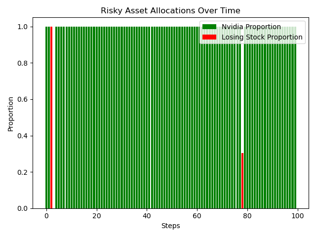
allocations = np.array(allocations)
plt.bar(range(num_steps),height=allocations[:, 0], label='Nvidia Proportion', color='green')
plt.bar(range(num_steps),height=allocations[:, 1], label='Losing Stock Proportion', color='red')
plt.title('Risky Asset Allocations Over Time')
plt.xlabel('Steps')
plt.ylabel('Proportion')
plt.legend()
plt.tight_layout()
plt.show()We can see in the graph how the porfolio value is greater than the simulation with no risk.
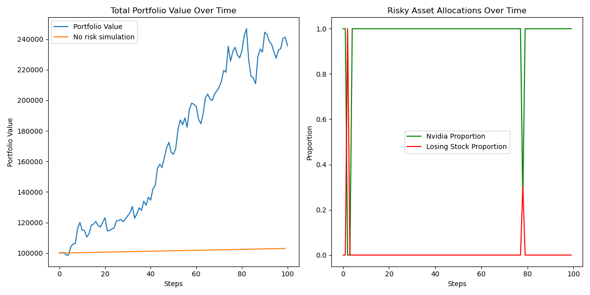
We can see the optimal policy is to put all your money in Nvidia asset most of the time.